Сэмплинг
Содержание:
- Oversampling
- When sampling is applied
- Carrier and Downconversion
- What Is a Sampling Error?
- Стратегии сэмплирования[править]
- Классификация методов сэмплинга
- Examples of Sampling Errors
- Sampling Distribution — Central Limit Theorem
- Quadrature Sampling
- Receiver Side
- Особенности применения сэмплинга
- Downsampling
- Top P sampling
- Мнения
- Sampling Distribution — What and Why
- Sampling from a probability distribution
- Мотивация
Oversampling
И децимацию и интерполяцию уже упомянули. Вроде бы и всё. Но в плагинах часто можно увидеть термин oversampling, да ещё и с каким-то настройками. Давайте разбираться.
Есть такое определение как «Дискретизация сигналов с запасом по частоте дискретизации». То есть применяется дискретизация сигнала на частоте, в несколько раз превышающей частоту Котельникова (предел Найквиста) с последующей децимацией. Вот она и называется в англоязычной литературе термином oversampling.
Например, возьмём сигнал с шириной полосы или самой высокой частотой B = 100 Гц. Зная, что есть предел Найквиста берётся частота дискретизации в 2 раза больше — 200 Гц (100 × 2). При oversampling 4x частота дискретизации в четыре раза превышает частоту дискретизации 800 Гц (200 × 4). В итоге фильтр anti — aliasing работает в переходной полосе 300 Гц. То есть получается следующая формула (( f s / 2) — B = (800 Гц / 2) — 100 Гц = 300 Гц.
Что даёт такой тип дискретизации сигнала?
- Возможность использовать АЦП (аналого-цифровой преобразователь) с меньшей разрядностью.
- Возможность использовать более простой и дешёвый аналоговый фильтр для защиты от наложения спектров.
- Подобная передискретизация способна улучшить разрешение и отношение сигнал / шум, а также может помочь избежать наложения спектров и фазовых искажений путем ослабления требований к характеристикам фильтра сглаживания.
Аналогичный подход применяется и при восстановлении сигнала по его отсчётам.
When sampling is applied
The following sections explain where you can expect session sampling in Analytics reports.
Default reports
Analytics has a set of preconfigured, default reports listed in the left pane under Audience, Acquisition, Behavior, and Conversions.
Analytics stores one complete, unfiltered set of data for each property in each account. For each reporting view in a property, Analytics also creates tables of aggregated dimensions and metrics from the complete, unfiltered data. When you run a default report, Analytics queries the tables of aggregated data to quickly deliver unsampled results.
Analytics periodically adds new reports, and sometimes makes changes to the way metrics are calculated. If the date range of a report includes a time before the report was added or before a metric calculation changed, then Analytics can issue an ad-hoc query, and the data might be sampled.
Data is sampled when reports that include the Users and Active Users metrics include data from before September 2016. Learn more
Default reports are unsampled in both Analytics Standard and Analytics 360. However, if you use the , you may experience sampling in some of your Google Ads reports.
Ad-hoc reports
If you modify a default report in some way—for example, by applying a segment, filter, or secondary dimension—or if you create a custom report with a combination of dimensions and metrics that don’t exist in a default report, you are generating an ad-hoc query of Analytics data.
Analytics first goes to the aggregated data tables to see if all of the requested information from your ad-hoc query is available there. If the information is not available there, Analytics queries the complete, unfiltered set of data to satisfy the query request.
Ad-hoc queries are subject to sampling if the number of sessions for the date range you are using exceeds the threshold for your property type.
The sampling algorithm uses a sample of the complete data that is proportional to the daily distribution of sessions for the property for the date range you’re using. For example, if over a 5-day period, sessions were sampled at 25%, then the sample would include 25% of each day’s sessions:
| Monday | Tuesday | Wednesday | Thursday | Friday | |
|---|---|---|---|---|---|
| Total sessions | 200,000 | 100,000 | 200,000 | 300,000 | 200,000 |
| 25% sample | 50,000 | 25,000 | 50,000 | 75,000 | 50,000 |
The sampling rate varies from query to query depending on the number of sessions during a date range for a given view.
When sampling is in effect, you see a message at the top of the report that says This report is based on N% of sessions.
To the right of that message, you can select one of two options to change the sampling size:
- Greater precision: Uses the maximum sample size possible to give you results that are the most precise representation of your full data set
- Faster response: Uses a smaller sampling size to give you faster results

Other reports
Sampling works differently for these reports than for default reports or ad-hoc queries.
Multi-Channel Funnels reports
Like default reports, no sampling is applied unless you modify the report—for example, by changing the lookback window, by changing which conversions are included, or by adding a segment or secondary dimension. If you modify the report in any way, a maximum sample of 1M conversions will be returned.
Flow-visualization reports
Flow-visualization reports (Users Flow, Behavior Flow, Events Flow, Goal Flow) are generated from a maximum of 100K sessions for the selected date range.
The flow-visualization reports, including entrance, exit, and conversion rates, may differ from the results in the default Behavior and Conversions reports, which are based on a different sample set.
Filters and segments
Analytics Standard and Analytics 360 sample session data at the view level, after view filters have been applied. For example, if view filters include or exclude sessions, then the sample is taken from only those sessions.
Analytics Standard and Analytics 360 both apply segments after applying report filters and after sampling, which means that a segment may include fewer sessions than are included in the overall sample.
Carrier and Downconversion
Until this point we have not discussed frequency, but we saw there was an in the equations involving the cos() and sin(). This frequency is the frequency of the sine wave we actually send through the air (the electromagnetic wave’s frequency). We refer to it as the “carrier” because it carries our information (stored in I and Q) on a certain frequency.

For reference, radio signals such as FM radio, WiFi, Bluetooth, LTE, GPS, etc., usually use a frequency (i.e., a carrier) between 100 MHz and 6 GHz. These frequencies travel really well through the air, but they don’t require super long antennas or a ton of power to transmit or receive. Your microwave cooks food with electromagnetic waves at 2.4 GHz. If there is a leak in the door then your microwave will jam WiFi signals and possibly also burn your skin. Another form of electromagnetic waves is light. Visible light has a frequency of around 500 THz. It’s so high that we don’t use traditional antennas to transmit light. We use methods like LEDs that are semiconductor devices. They create light when electrons jump in between the atomic orbits of the semiconductor material, and the color depends on how far they jump. Technically, radio frequency (RF) is defined as the range from roughly 20 kHz to 300 GHz. These are the frequencies at which energy from an oscillating electric current can radiate off a conductor (an antenna) and travel through space. The 100 MHz to 6 GHz range are the more useful frequencies, at least for most modern applications. Frequencies above 6 GHz have been used for radar and satellite communications for decades, and are now being used in 5G “mmWave” (24 — 29 GHz) to supplement the lower bands and increase speeds.
When we change our IQ values quickly and transmit our carrier, it’s called “modulating” the carrier (with data or whatever we want). When we change I and Q, we change the phase and amplitude of the carrier. Another option is to change the frequency of the carrier, i.e., shift it slightly up or down, which is what FM radio does.
As a simple example, let’s say we transmit the IQ sample 1+0j, and then we switch to transmitting 0+1j. We go from sending to , meaning our carrier shifts phase by 90 degrees when we switch from one sample to another.
Now back to sampling for a second. Instead of receiving samples by multiplying what comes off the antenna by a cos() and sin() then recording I and Q, what if we fed the signal from the antenna into a single analog-to-digital converter, like in the direct sampling architecture we just discussed? Say the carrier frequency is 2.4 GHz, like WiFi or Bluetooth. That means we would have to sample at 4.8 GHz, as we learned. That’s extremely fast! An ADC that samples that fast costs thousands of dollars. Instead, we “downconvert” the signal so that the signal we want to sample is centered around DC or 0 Hz. This downconversion happens before we sample. We go from:
to just I and Q.
Let’s visualize downconversion in the frequency domain:

When we are centered around 0 Hz, the maximum frequency is no longer 2.4 GHz but is based on the signal’s characteristics since we removed the carrier. Most signals are around 100 kHz to 40 MHz wide in bandwidth, so through downconversion we can sample at a much lower rate. Both the B2X0 USRPs and PlutoSDR contain an RF integrated circuit (RFIC) that can sample up to 56 MHz, which is high enough for most signals we will encounter.
What Is a Sampling Error?
A sampling error is a statistical error that occurs when an analyst does not select a sample that represents the entire population of data. As a result, the results found in the sample do not represent the results that would be obtained from the entire population.
Sampling is an analysis performed by selecting a number of observations from a larger population. The method of selection can produce both sampling errors and non-sampling errors.
Key Takeaways
- A sampling error occurs when the sample used in the study is not representative of the whole population.
- Sampling is an analysis performed by selecting a number of observations from a larger population.
- Even randomized samples will have some degree of sampling error because a sample is only an approximation of the population from which it is drawn.
- The prevalence of sampling errors can be reduced by increasing the sample size.
- Random sampling is an additional way to minimize the occurrence of sampling errors.
- In general, sampling errors can be placed into four categories: population-specific error, selection error, sample frame error, or non-response error.
Стратегии сэмплирования[править]
- Cубдискретизация (англ. under-sampling) — удаление некоторого количества примеров мажоритарного класса.
- Передискретизации (англ. over-sampling) — увеличение количества примеров миноритарного класса.
- Комбинирование (англ. сombining over- and under-sampling) — последовательное применение субдискретизации и передискретизации.
- Ансамбль сбалансированных наборов (англ. ensemble balanced sets) — использование встроенных методов сэмплирования в процессе построения ансамблей классификаторов.
Также все методы можно разделить на две группы: случайные (недетерминированные) и специальные (детерминированные).
- Случайное сэмплирование (англ. random sampling) — для этого типа сэмплирования существует равная вероятность выбора любого конкретного элемента. Например, выбор 10 чисел в промежутке от 1 до 100. Здесь каждое число имеет равную вероятность быть выбранным.
- Сэплирование с заменой (англ. sampling with replacement) — здесь элемент, который выбирается первым, не должен влиять на вторую или любую другую выборку. Математически, ковариация равна нулю между двумя выборками. Мы должны использовать выборку с заменой, когда у нас большой набор данных. Потому что, если мы используем выборку без замены, то вероятность для каждого предмета, который будет выбран, будет изменяться, и она будет слишком сложной после определенного момента. Выборка с заменой может сказать нам, что чаще встречается в наших данных.
- Сэмплирование без замены (англ. sampling without replacement) — здесь то, что мы выбираем первым, повлияет на второе. Выборка без замены полезна, если набор данных мал. Математически, ковариация между двумя выборками не равна нулю.
- Стратифицированное сэмплирование (англ. stratified sampling) — в этом типе техники мы выбираем из определенной группы объектов из всей выборки. Из каждой группы извлекается одинаковое количество объектов, хотя группы имеют разные размеры. Кроме того, существует вариант, когда количество объектов, выбранных из каждой группы, пропорционально размеру этой группы.
Классификация методов сэмплинга
Общепринятая классификация методов сэмплинга представлена на рис. 2.
Рисунок 2. Классификация методов сэмплинга
Все методы сэмплинга делятся на две группы — детерминированные и вероятностные (probability sampling) или случайные (random sampling). В детерминированных методах процесс формирования выборки производится в соответствии с формально заданными правилами и ограничениями. Например «выбрать всех мужчин в возрасте от 30 до 40 лет». Тогда все объекты, удовлетворяющие правилу будут помещены в выборку обязательно. В вероятностных методах для каждого объекта определяется вероятность, с которой он может быть взят в выборку.
Examples of Sampling Errors
Assume that XYZ Company provides a subscription-based service that allows consumers to pay a monthly fee to stream videos and other types of programming via an Internet connection.
The firm wants to survey homeowners who watch at least 10 hours of programming via the Internet per week and that pay for an existing video streaming service. XYZ wants to determine what percentage of the population is interested in a lower-priced subscription service. If XYZ does not think carefully about the sampling process, several types of sampling errors may occur.
A population specification error would occur if XYZ Company does not understand the specific types of consumers who should be included in the sample. For example, if XYZ creates a population of people between the ages of 15 and 25 years old, many of those consumers do not make the purchasing decision about a video streaming service because they may not work full-time. On the other hand, if XYZ put together a sample of working adults who make purchase decisions, the consumers in this group may not watch 10 hours of video programming each week.
Selection error also causes distortions in the results of a sample. A common example is a survey that only relies on a small portion of people who immediately respond. If XYZ makes an effort to follow up with consumers who don’t initially respond, the results of the survey may change. Furthermore, if XYZ excludes consumers who don’t respond right away, the sample results may not reflect the preferences of the entire population.
Sampling Distribution — Central Limit Theorem
The outcome of our simulation shows a very interesting phenomenon: the sampling distribution of sample means is very different from the of marriages over 976 inhabitants: the sampling distribution is much less skewed (or more symmetrical) and smoother.
In fact, means and sums are always (approximately) for reasonable sample sizes, say n > 30. This doesn’t depend on whatever population distribution the data values may or may not follow. This phenomenon is known as the central limit theorem.
Note that even for 1,000 samples of n = 10, our sampling distribution of means is already looking somewhat similar to the normal distribution shown below.
Quadrature Sampling
The term “quadrature” has many meanings, but in the context of DSP and SDR it refers to two waves that are 90 degrees out of phase. Why 90 degrees out of phase? Consider how two waves that are 180 degrees out of phase are essentially the same wave with one multiplied by -1. By being 90 degrees out of phase they become orthogonal, and there’s a lot of cool stuff you can do with orthogonal functions. For the sake of simplicity, we use sine and cosine as our two sine waves that are 90 degrees out of phase.
Next let’s assign variables to represent the amplitude of the sine and cosine. We will use for the cos() and for the sin():
We can see this visually by plotting I and Q equal to 1:
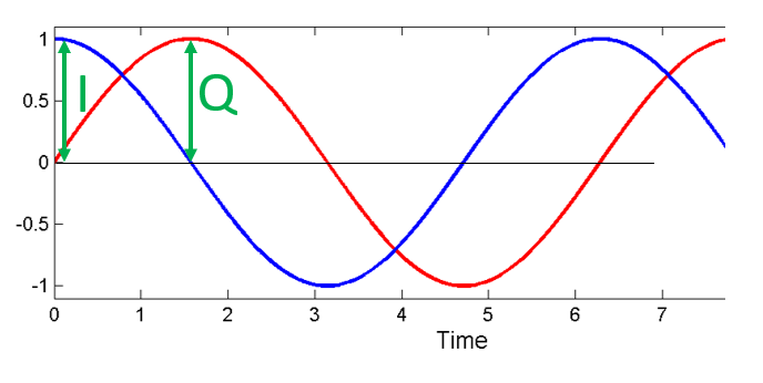
We call the cos() the “in phase” component, hence the name I, and the sin() is the 90 degrees out of phase or “quadrature” component, hence Q. Although if you accidentally mix it up and assign Q to the cos() and I to the sin(), it won’t make a difference for most situations.
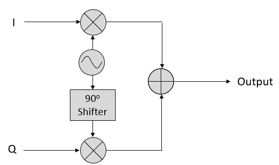
IQ sampling is more easily understood by using the transmitter’s point of view, i.e., considering the task of transmitting a RF signal through the air. What we do as the transmitter is add the sin() and cos(). Let’s say x(t) is our signal to transmit:
What happens when we add a sine and cosine? Or rather, what happens when we add two sinusoids that are 90 degrees out of phase? In the video below, there is a slider for adjusting I and another for adjusting Q. What is plotted are the cosine, sine, and then the sum of the two.

(The code used for this pyqtgraph-based Python app can be found here)
The important take-aways are that when we add the cos() and sin(), we get another pure sine wave with a different phase and amplitude. Also, the phase shifts as we slowly remove or add one of the two parts. The amplitude also changes. This is all a result of the trig identity: , which we will come back to in a bit. The “utility” of this behavior is that we can control the phase and amplitude of a resulting sine wave by adjusting the amplitudes I and Q (we don’t have to adjust the phase of the cosine or sine). For example, we could adjust I and Q in a way that keeps the amplitude constant and makes the phase whatever we want. As a transmitter this ability is extremely useful because we know that we need to transmit a sinusoidal signal in order for it to fly through the air as an electromagnetic wave. And it’s much easier to adjust two amplitudes and perform an addition operation compared to adjusting an amplitude and a phase. The result is that our transmitter will look something like this:
Receiver Side
Now let’s take the perspective of a radio receiver that is trying to receive a signal (e.g., an FM radio signal). Using IQ sampling, the diagram now looks like:
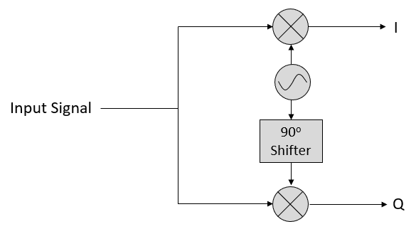
What comes in is a real signal received by our antenna, and those are transformed into IQ values. What we do is sample the I and Q branches individually, using two analog-to-digital converters (ADCs), and then we combine the pairs and store them as complex numbers. In other words, at each time step, you will sample one I value and one Q value and combine them in the form (i.e., one complex number per IQ sample). There will always be a “sample rate”, the rate at which sampling is performed. Someone might say, “I have an SDR running at 2 MHz sample rate.” What they mean is that the SDR receives two million IQ samples per second.
If someone gives you a bunch of IQ samples, it will look like a 1D array/vector of complex numbers. This point, complex or not, is what this entire chapter has been building to, and we finally made it.
Throughout this textbook you will become very familiar with how IQ samples work, how to receive and transmit them with an SDR, how to process them in Python, and how to save them to a file for later analysis.
Особенности применения сэмплинга
Кроме выбора собственно метода сэмплинга, который наилучшим образом подходит к решаемой задаче и используемым данным, аналитику требуется принять решение о некоторых особенностях его применения. Обычно это связано с выбором, будет ли реализован сэмплинг с возвратом или без, а также определить размер полученной выборки.
Сэмплинг с возвратом (заменой) — это методика построения выборок, при которой каждый объект исходной совокупности может быть выбран более, чем один раз. Т.е. предполагается что отбираемый объект не перемещается, а копируется в выборку, оставаясь в исходной совокупности.
Сэмплинг без возврата (замены) предполагает, что каждый объект совокупности может быть выбран только один раз. Т.е. объект перемещается из исходной совокупности в выборку.
Сэмплинг с возвратом используется в том случае, если количество уникальных объектов совокупности недостаточно для формирования выборки требуемого объема, что компенсируется возможностью многократного выбора объектов. Недостатком подхода является появление в выборке дубликатов. Таким образом, сэмплинг с заменой позволяет увеличить объем выборки, но не её репрезентативность.
Определение объёма выборки. Определение числа объектов, из которого будет состоять выборка, является важным элементом любого эмпирического исследования в статистике или анализе данных, по результатам которого должны быть сделаны вывод о свойствах совокупности на основе свойств выборки.
На практике объём выборки обычно определяется на основе затрат, времени или удобства сбора данных, а также необходимости достижения необходимой репрезентативности и полноты.
В заключении следует отметить, что несмотря на общепринятую схему классификации, которая наиболее часто приводится в литературе, методология сэмплинга не имеет чётких границ. Вообще говоря, к сэмплингу можно отнести любой метод отбора данных, который формирует выборки, с помощью которых пользователь может решать свои задачи. Например, в сэмплинге могут использоваться алгоритмы фильтрации строк.
При этом достижение репрезентативности, полноты и точности выборки не является приоритетным. Главное, чтобы она была полезной для решения практической задачи. Вопрос только в корректности построенных с её помощью моделей, сделанных выводах и обобщениях.
Другие материалы по теме:
Downsampling
Итак, при уменьшении частоты дискретизации упрощённо происходит два этапа:
- Цифровая фильтрация сигнала для того, чтобы удалить высокочастотные составляющие, которые не удовлетворяют пределу Найквиста для новой частоты дискретизации;
- Удаление или (отбрасывание) лишних отсчетов (сохраняется каждый N-й отсчёт). Здесь следует пояснить, что при программной реализации алгоритма децимации «лишние» отсчёты не удаляются, а просто не вычисляются (отбрасываются). При этом число обращений к цифровому фильтру уменьшается в определённое количество раз.
Так вот. Второй этап удаление или (отбрасывание) лишних отсчетов в англоязычной литературе иногда обозначают термином downsampling, что по сути может употребляться как синоним термина «децимация».
Top P sampling
Another way to exclude very low probability tokens is to include the most probable tokens that make up the “nucleus” of the PMF, such that the sum of the most probable tokens just reaches p. For example, suppose we set p = 0.75; with Top P sampling, we would include the most probable next tokens until the cumulative probability until the sum reaches 0.75, at which point we stop including tokens.
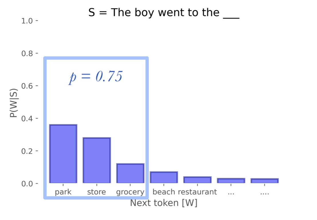
Here, we consider park, store, and grocery, because those three satisfy our probability threshold of 0.75
This has the advantage of being flexible as the distribution changes, allowing the size of the filtered words to expand and contract when it makes sense.
Мнения
Заместитель генерального директора ОАО «КапиталЪ Страхование» Дмитрий Боткин:
Сэмплинг страховых услуг может эффективно работать на больших массивах страхователей. Предложение бесплатных, «на пробу» страховых услуг в торговых центрах не окупает вложенных затрат: не та целевая аудитория. Сегодня страховщики собрали большие базы данных только по ОСАГО, и это опять-таки не та целевая аудитория. По этим базам число обратившихся в страховую компанию по рассылке методом директ-маркетинга не превысит 1%, а купят страховой полис еще меньше. Сэмплинг может хорошо работать только на массивах потенциальных страхователей с откликом не ниже 10%, а это уже хорошо подготовленная к финансовым услугам аудитория, которая пока есть только у банков. Вопрос только в том, готовы ли банки поделиться своими клиентами со страховщиками.
Директор по маркетингу группы «Альфа-Страхование» Евгений Белобородов:
Одна из основных причин, по которым сэмплинг не может быть в полной мере применен к страхованию, сводится к стоимости страхового продукта и циклу его потребления. Цикл потребления пищевых продуктов обычно составляет несколько дней. Распробовав йогурт или сок, человек очень быстро начинает совершать покупки за свой счет. В страховании же стандартный цикл потребления равен одному году. Стоимость упаковки йогурта, стакана сока, даже недельного пропуска в тренажерный зал или открытого тест-драйва просто несравнима с возможными затратами страховщика на восстановление автомобиля клиента после серьезной аварии и оплату лечения водителя при полученных травмах. Разбрасываться такими дорогими подарками страховым компаниям невыгодно.
Недельный же полис страхования не дает клиенту представления о страховом продукте — для этого надо, как минимум, успеть получить страховое возмещение, а вероятность наступления страхового события в недельный срок крайне мала: почувствовать «вкус» продукта практически невозможно.
Генеральный директор «Русской страховой компании» Геннадий Смирнов:
Недостаточное развитие сэмплинга в страховании, то есть бесплатных полисов, может быть связано с особенностями ведения бухгалтерского учета и налогообложения страховых компаний. Страховщику в случае выдачи бесплатного страхового полиса придется формировать страховые резервы за свой счет, из прибыли, что сильно повышает цену сэмплинг-акции. Правда, есть еще один способ, но он не приветствуется. Это оформить бесплатные полисы как платные за счет «серых» средств.
Генеральный директор СК «МРСС» Семен Акерман:
Подарки, которые дарит страховая компания, должны быть со смыслом и отражать сущность страхования. Тогда такая акция будет максимально стремиться к сэмплингу. Очень удачный пример встретился мне в Германии. Одна из страховых компаний делала подарок в виде молотка для разбивки лобового стекла при ДТП. Слоган у этой компании звучал примерно так: «В трудной ситуации мы думаем о вас». Понятно, что и молоток, и страхование имели своей целью «протянуть страхователю руку помощи в трудной ситуации».
Но в этом деле главное — не перегнуть палку. А то будем дарить бейсбольные биты с надписью «Всем врагам BMW посвящается».
Д.Брызгалов
Независимый эксперт
Sampling Distribution — What and Why
The government has these exact population figures. However, a social scientist doesn’t have access to these data. So although the government knows, our scientist is clueless how often the island inhabitants marry. In theory, he could ask all 976 people and thus find the exact population distribution of marriages. Since this is too time consuming, he decides to draw a simple random sample of n = 10 people.
On average, the 10 respondents married 1.1 times. So what does this say about the entire population of 976 people? We can’t conclude that they marry 1.1 times on average because a second sample of n = 10 will probably come up with a (slightly) different mean number of marriages.
This is basically the fundamental problem in inferential statistics: sample statistics vary over (hypothetical) samples. The solution to the problem is to figure out how much they vary. Like so, we can at least estimate a likely range -known as a confidence interval- for a population parameter such as an average number of marriages.
Sampling from a probability distribution
As a warm-up, let’s think for a minute how we might sample from a multinomial distribution with \(k\) possible outcomes and associated probabilities \(\theta_1, \dotsc, \theta_k\).
Sampling, in general, is not an easy problem. Our computers can only generate samples from very simple distributionsEven those samples are not truly random. They are actually taken from a deterministic sequence whose statistical properties (e.g., running averages) are indistinguishable from a truly random one. We call such sequences pseudorandom., such as the uniform distribution over \(\). All sampling techniques involve calling some kind of simple subroutine multiple times in a clever way.
In our case, we may reduce sampling from a multinomial variable to sampling a single uniform variable by subdividing a unit interval into \(k\) regions with region \(i\) having size \(\theta_i\). We then sample uniformly from \(\) and return the value of the region in which our sample falls.
Reducing sampling from a multinomial distribution to sampling a uniform distribution in .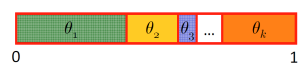
Forward Sampling
⊕
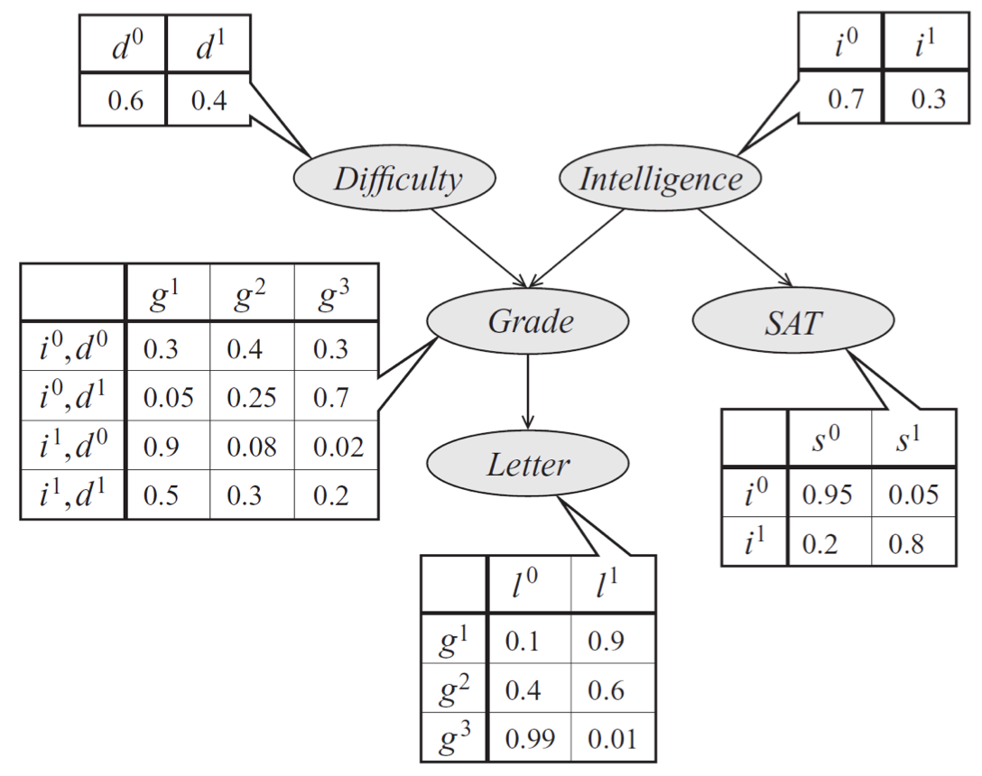
Bayes net model describing the performance of a student on an exam. The distribution can be represented a product of conditional probability distributions specified by tables.
Our technique for sampling from multinomials naturally extends to Bayesian networks with multinomial variables, via a method called ancestral (or forward) sampling. Given a probability \(p(x_1, \dotsc, x_n)\) specified by a Bayes net, we sample variables in topological order. We start by sampling the variables with no parents; then we sample from the next generation by conditioning these variables’ CPDs to values sampled at the first step. We proceed like this until all \(n\) variables have been sampled. Importantly, in a Bayesian network over \(n\) variables, forward sampling allows us to sample from the joint distribution \(\bfx \sim p(\bfx)\) in linear \(O(n)\) time by taking exactly 1 multinomial sample from each CPD.
In our earlier model of a student’s grade, we would first sample an exam difficulty \(d’\) and an intelligence level \(i’\). Then, once we have samples \(d’\) and \(i’\), we generate a student grade \(g’\) from \(p(g \mid d’, i’)\). At each step, we simply perform standard multinomial sampling.
A former CS228 student has created an interactive web simulation for visualizing Bayesian network forward sampling methods. Feel free to play around with it and, if you do, please submit any feedback or bugs through the Feedback button on the web app.
“Forward sampling” can also be performed efficiently on undirected models if the model can be represented by a clique tree with a small number of variables per node. Calibrate the clique tree, which gives us the marginal distribution over each node, and choose a node to be the root. Then, marginalize over variables in the root node to get the marginal for a single variable. Once the marginal for a single variable \(x_1 \sim p(X_1 \mid E=e)\) has been sampled from the root node, the newly sampled value \(X_1 = x_1\) can be incorporated as evidence. Finish sampling other variables from the same node, each time incorporating the newly sampled nodes as evidence, i.e., \(x_2 \sim p(X_2=x_2 \mid X_1=x_1,E=e)\) and \(x_3 \sim p(X_3=x_3 \mid X_1=x_1,X_2=x_2,E=e)\) and so on. When moving down the tree to sample variables from other nodes, each node must send an updated message containing the values of the sampled variables.
Мотивация
Сглаживание проявляется в случае 2D-изображений в виде муара и пиксельных краев, в просторечии известных как « неровности ». Общие обработки сигналов и обработка изображений знания предполагают , что для достижения идеального устранения наложения спектров , надлежащие пространственный отбора проб на Найквист скорости (или выше) после применения 2D сглаживающего фильтра не требуются. Поскольку этот подход потребовал бы прямого и обратного преобразования Фурье , были разработаны менее требовательные в вычислительном отношении приближения, такие как суперсэмплинг, чтобы избежать переключений областей, оставаясь в пространственной области («области изображения»).